NGPConv - Scaling 3D ConvNets to gigavoxel images using Implicit Neural Representations
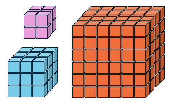
Table of Contents
- TL;DR
- Introduction
- Implicit Neural Representations
- Instant NGP
- Convolutional Neural Networks on Instant NGP Representations
- CUDA implementation
- Performance Benchmark
- Conclusion
TL;DR
3D ConvNets are limited to low resolution images due to the cubic scaling of the number of voxels. However, applications like medical imaging, weather forecasting, high-fidelity scene representations, etc. require ultra high resolution images on which 3D ConvNets run out of memory 😓
To scale 3D ConvNets to gigavoxel images, we use InstantNGP to compress the data into an implicit codebook and define a convolution operator on the codebook itself. Our CUDA kernel is up to 10x faster than a PyTorch implementation 🚀🚀
Introduction
Convolutional architectures have been the backbone of computer vision and natural language processing. Even with the domination of transformer models from large language models, convolutional networks have stayed competitive for visual processing. Although standard 2D convolutional architectures support very high resolution 2D images (upto 4k images), 3D convolutional networks have have been limited to lower resolutions.
Although 3D convolutional networks are ubiquitiously used in fields like medical imaging, they have been limited to lower resolutions. For example, the 3D convolutional architectures in VoxelMorph, SynthSeg and nnUNet have been limited to smaller resolutions like $160\times 192\times 224$ or $128\times 128\times 128$. This is because the number of activations in convolutional architecture is proportional to the number of voxels in the input volume.
Larger datasets like the CCFv3 Atlas have resolutions of upto $1320\times 1140\times 800$ voxels, BigBrain has $1700 \times 1600 \times 1300$ voxels, more than $500$ times larger than the current capacity of 3d deep learning models. Even a single 3D convolutional layer with 32 hidden dimensions would generate an activation volume of size 420GB. This is not feasible for current hardware.
📝 Note: In this blog, I will use medical images as a representative example, but other representations like NeRFs, signed distance fields (SDFs), or occupancy fields are also represented by regular grids, but consume a lot of memory due to the cubic scaling of the number of voxels.
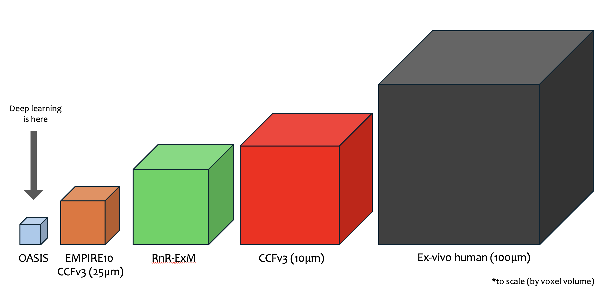
Figure: Most Deep Learning models are trained on small 3D datasets like OASIS. On the contrary, large datasets like CCFv3 and BigBrain are out of reach for current deep learning models.
There is a resolution – computation tradeoff. To work with high resolution voxel grids (medical images, 3D scene representations) or densely sampled point clouds, we have to sacrifice network capacity. Fortunately, most of the information stored in the representation is highly redundant. This motivates the use of implicit neural representations.
Implicit Neural Representations
Implicit Neural Representations (INRs) are a class of models that represent high-dimensional data as a function of the coordinates. The function is typically represented as a neural network that takes in the coordinates and outputs a scalar value. The scalar value is then used to compute the color and opacity of the pixel. For redundant data, the data is encoded succintly in the weights of the neural network.
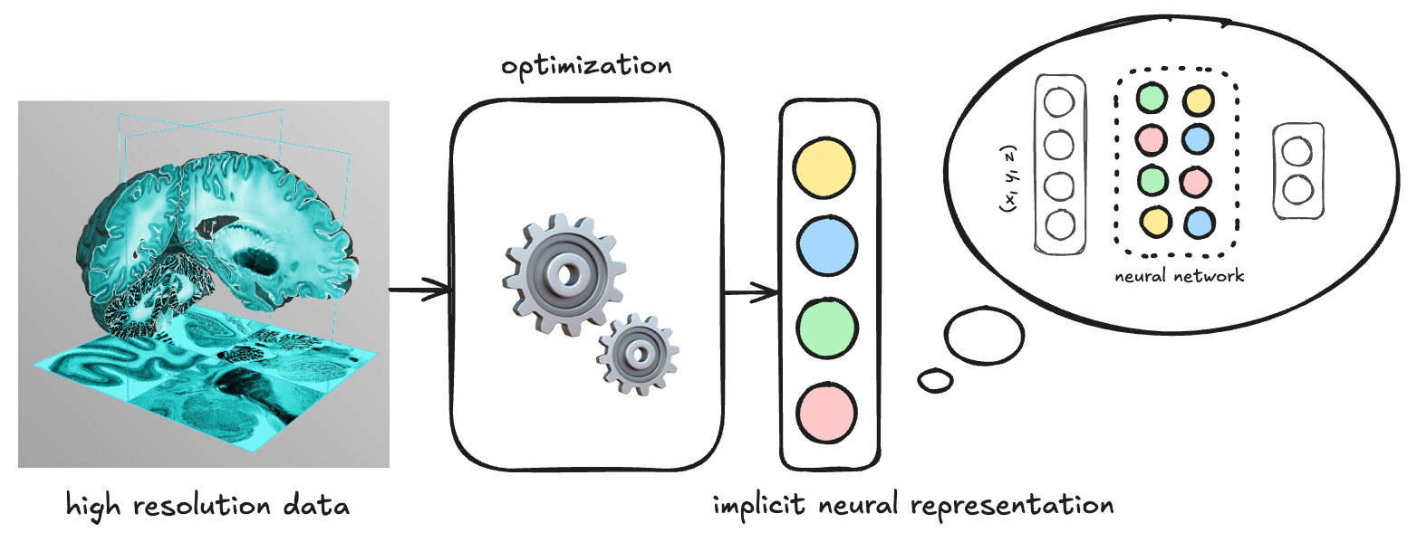
Figure: The data (brain on left) is encoded into an implicit neural representation (colored neurons on the right). The representation is typically weights of a neural network which resolved a coordinate to a scalar or vector value corresponding to the data.
In principle, a neural network can then process the encoded data for downstream tasks.
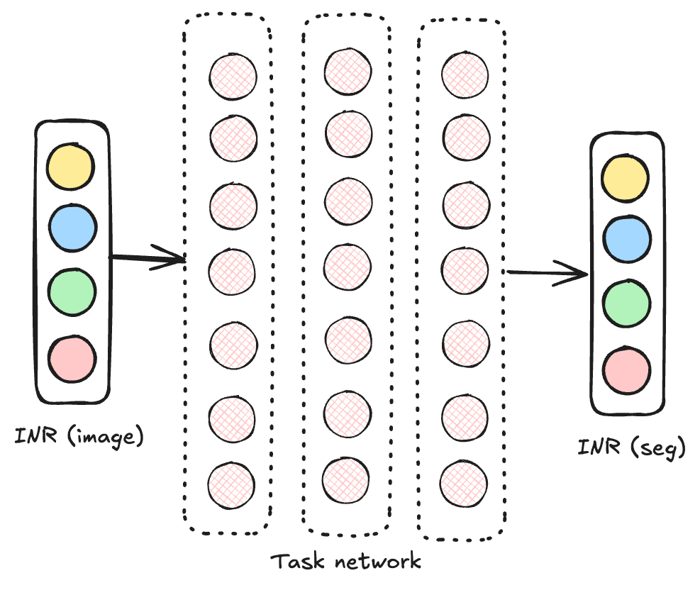
Figure: A typical network operating on the implicit representation would take the INR of the image as input, and emit the INR of the segmentation map as output. If the network operates entirely in the INR space, it can work with larger images out of the box.
However, there are two main challenges with the formulation above:
- The implicit representation has no spatial locality unlike the data that it represents since all nodes encode the data at all locations. This makes it difficult to leverage the inductive bias of the original data (which is why we use convolutional networks in the first place).
- The INR representations for different images do not share the same basis functions. The neural representation might encode data differently for different images – making it hard for a downstream network to infer the basis functions used to encode the data.
Instant NGP
Instant NGP was proposed to represent high resolution data like gigapixel images, signed distance fields, and NeRFs using an implicit representation. The idea is to use a hash function that converts quantized spatial coordinates to a set of indices that are used to index into a codebook. This is done across multiple resolutions and the codebook entries are concatenated together to form a single vector for a given coordinate. The vector is then fed into an MLP decoder to get the final output. The codebook and decoder are trained end-to-end to minimize the reconstruction loss.
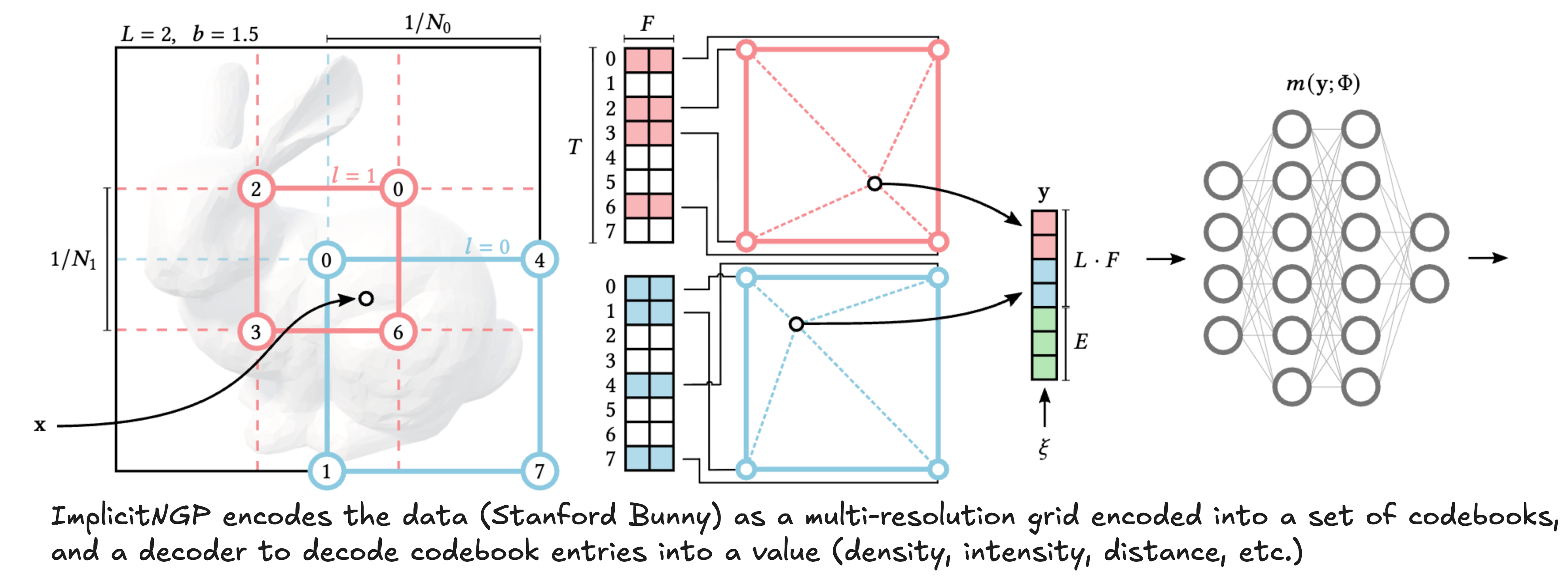
Figure: Architecture of Instant NGP. Unlike other neural representations, this representation has some spatial locality since only a few fixed entries of the codebook are used for a given coordinate, solving our first problem. To solve the second problem, we initialize a different codebook for each image (which forms our implicit representation), and use a shared MLP decoder (see below).
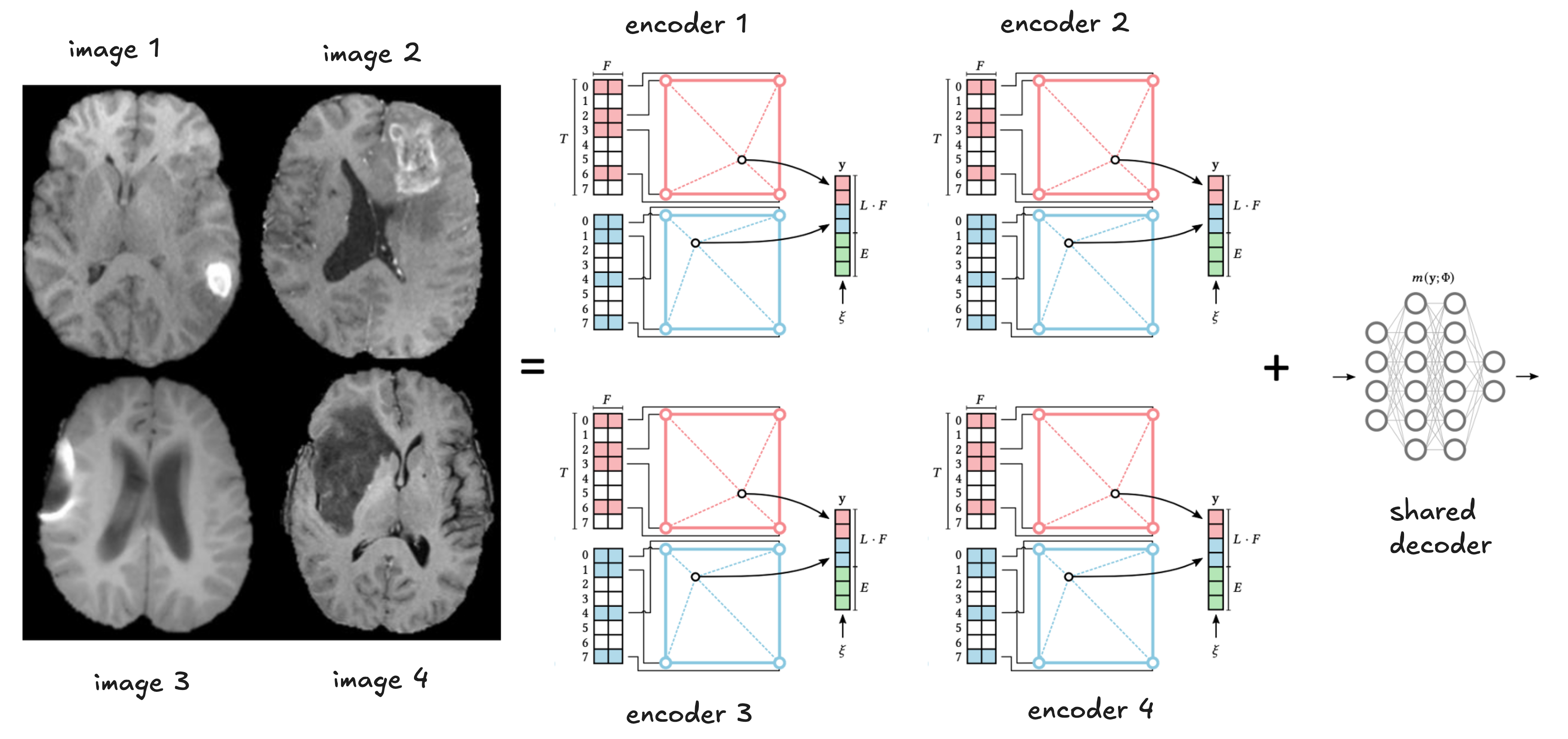
Figure: The codebooks are initialized with random weights, and the decoder is shared across all codebooks.
This design ensures that different images are decoded the same way, solving our second problem – now multiple codebooks lie in the same encoded space. Given a dataset of $N$ images, we perform a joint optimization of $N$ codebooks and a shared MLP decoder to encode the data.
This deviates from how Implicit Neural Representations are typically trained, where a single datum is considered at a time. However, this idea allows compressing the data into a spatially local representation amenable to convolutional operations.
Does joint optimization regress performance?
📝 Note: I’m using 3D images from the BRATs brain MRI dataset as a representative example. But other data like scene representations, NeRFs, SDFs, can be used as well.
The first experiment is to train $N$ encoders and a single decoder jointly.
My intuition was that as we add more encoders and a single decoder, the reconstruction performance would degrade. However, I saw quite the opposite trend - the average PSNR of the reconstructions improved as we added more encoders.
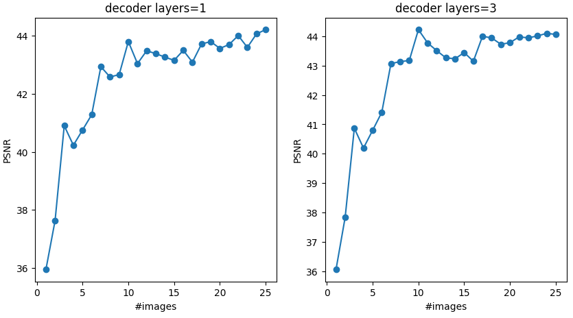
Figure: The average PSNR of the reconstructions improves as we add more encoders.
This is an interesting result, suggesting that the decoder is not throttled by the number of encoders, but rather leverages shared knowledge across the different codebooks to reconstruct each datum better.
I suspected some images might be easier to learn than others and might be skewing this plot, so I plotted the PSNR for each image individually.
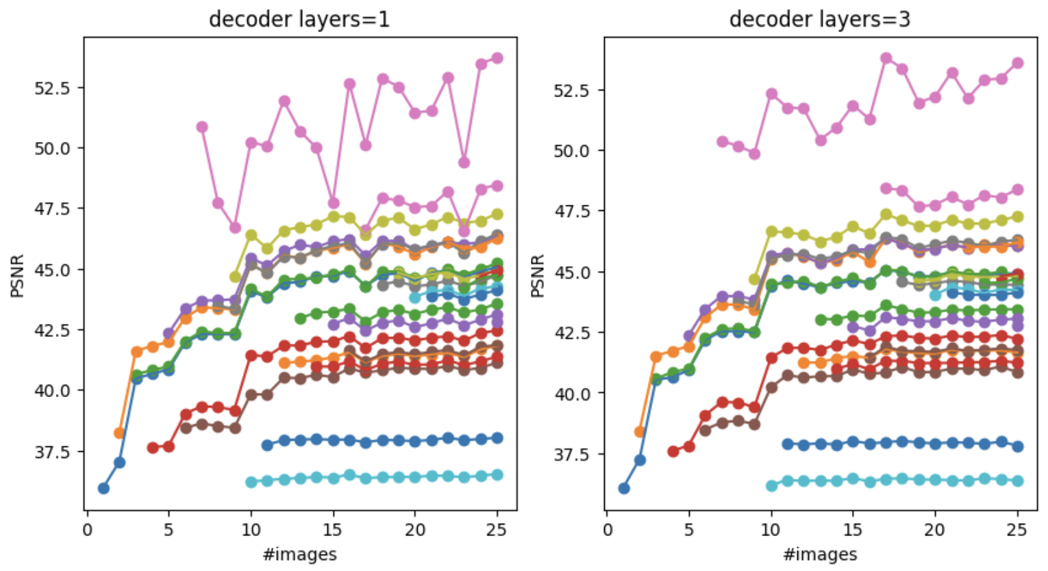
Figure: The PSNR of the reconstructions for each image individually. Almost all images benefit from training with more encoders.
Indeed, some images are easier to learn than others (as seen by the different PSNR bands), but most of the PSNR plots go up as we add more encoders. Even the “worst” images have a PSNR of more than 35dB!!
This is the first promising result - we are not losing reconstruction performance as the dataset size increases, in fact, quite the contrary.
Convolutional Neural Networks on Instant NGP codebooks
The second (and more interesting) piece of the puzzle is to actually define the convolutional operator on the implicit representation. This is where we dive into the dirty details.
The coordinate encoding
The data or scene is assumed to live inside a continuous bounding box $x_0 \in \mathcal{B} = [0, 1]^d$. The implicit representation defines a set of levels with resolutions $L_1, L_2, \ldots, L_K$. At level $k$, the input space $\mathcal{B}$ is quantized to a regular grid of size $L_k^d$, and the feature vector at a location $x_k = L_k x_0$ is computed using bilinear interpolation from the values at the 8 nearest grid points.
Random hash function
The index in the codebooks for a quantized grid location $q$ is computed as:
\[h_k(q) = \left( \bigoplus_{i=1}^{d} q(i) \pi_i \right) \bmod T,\]where $\pi$ is the set of pre-determined prime numbers, $q(i)$ is the $i$-th coordinate of the quantized grid location $q$, and $T$ is the total number of codebook entries.
Tiled hash function
Another alternative hash function is to simply compute the flattened index of the quantized grid location $q$ as:
\[h_k(q) = \left( \sum_{i=1}^{d} q(i) L_k^{(i-1)} \right) \bmod T,\]Convolution operator
Recall that the convolution operator is defined as:
\[g(q) = \sum_{i=1}^{d} w(\Delta q) f(q - \Delta q),\]where $w$ is the kernel function and $f$ is the input feature map, and $\Delta q$ is the difference between the neighboring locations.
For a tiled hash function, note that if $s = h(q)$ is the entry corresponding to location $q$, then the hash for the neighboring locations $q + \Delta q$ is given by:
\[\begin{align*} h(q + \Delta q) &= \left( \sum_{i=1}^{d} (q(i) + \Delta q(i)) L_k^{(i-1)} \right) \bmod T \\ &= \left( \sum_{i=1}^{d} q(i) L_k^{(i-1)} + \sum_{i=1}^{d} \Delta q(i) L_k^{(i-1)} \right) \bmod T \\ &= \big(s + h(\Delta q)\big) \bmod T \end{align*}\]📝 Note: The hash function for the neighbors of a location $q$ are simply constant offsets $h(\Delta q)$ added to the hash of the original location $q$.
Therefore, the convolution for a input codebook $f$ at location $s$ can be computed as:
\[g(s) = \sum_{i=1}^{d} w(\Delta q) f((s + h(\Delta q)) \bmod T)\]Unlike in convolution over a spatially regular grid, the 3D `convolution’ here is actually performed on a 1D codebook with irregular (but constant) offsets determined by the hash function. This motivates the use of a fast convolution operator on the Implicit Neural Representations.
CUDA implementation
Now that we got the math out of the way, let’s implement the convolution operator in CUDA. The code is available here.
First, we need to convert a 3D quantized coordinate to a hash index using the tiled hash function.
1
2
3
4
5
6
__device__ __forceinline__ int compute_ravel_hash(const int *coord, const int resolution, const int hashmap_size) {
    // compute hash function for tiled grid
    int index;
    index = coord[0] + resolution*(coord[1] + resolution*coord[2]);
    return modpow2(index, hashmap_size);
}
We also compute the hash values for the neighboring locations.
1
2
3
4
5
6
__device__ __forceinline__ int compute_diff_hash(const int k1, const int k2, const int k3, const int lvl_res, const int hashmap_size) {
    int index = k1 + lvl_res*(k2 + lvl_res*k3);
    if(index >= 0)
        return index;
    return (hashmap_size - (modpow2(-index, hashmap_size)));
}
Note that the neighboring coordinates and the corresponding hash offset index can be negative (say for e.g. $\Delta q = (k_1, k_2, k_3) = (-1, -1, -1)$). If the index $h(\Delta q)$ is negative, we need to compute the value
using the fact that $-h(\Delta q)$ is positive, and computing the value in red.
Now let’s dive into the core logic of the forward pass of the convolution operator.
1
2
3
4
5
6
7
8
9
10
11
12
13
14
15
16
17
18
19
20
21
22
23

    CUDA_KERNEL_LOOP(index, num_outputs) {
        // get n, batch index, and output channel index
        // int c_out = index % output_channels;
        int c_out = modpow2(index, output_channels);    // assume channels are powers of 2
        int ibyout = divpow2(index, output_channels);
        int b_idx = modpow2(ibyout, batch_size);
        int n_idx = divpow2(ibyout, batch_size);
        // get level information
        int level = get_level(offsets_shared, n_idx, num_levels);
        int offset_lvl = offsets_shared[level];
        int local_n = n_idx - offset_lvl;
        int lvl_res = resolutions_shared[level];
        int lvl_res3 = lvl_res*lvl_res*lvl_res;
        // if this is a tail end, skip t
        if(local_n >= lvl_res3)
            continue;
        // now we have n, b, c --> time to get y[n, b, cout]
        scalar_t res = 0;
        int weight_index = level*kernel_volume*iosize + c_out;
        // cache this result in the beginning
        int coordstart[3];
        unravel_index(local_n, lvl_res, coordstart);
This code simply resolves the thread index index into the batch index b_idx, channel index c_out and the codebook entry index n_idx. The global index n_idx is resolved into a local codebook index local_n and the level level of the codebook. Finally, we unravel (x, y, z) = local_n to start the convolution.
The actual convolution is simply a loop
1
2
3
4
5
6
7
8
9
10
11
12
int fwd_index = n_idx * kernel_volume;   // set to n_idx, and loop over all kernel indices
for(int k1idx=0; k1idx<K1; k1idx++) {
    int k1 = k1idx - K1/2;
    for(int k2idx=0; k2idx<K2; k2idx++) {
        int k2 = k2idx - K2/2;
        for(int k3idx=0; k3idx<K3; k3idx++) {
            int k3 = k3idx - K3/2;
            // get neighboring index
            ...
        }
    }
}
This is simply a loop over the kernel indices $(k_1, k_2, k_3)$. Note that we do not perform tiling operations since the actual codebook entries are not spatially colocated. A tiled implementation using shared memory is also present in the code, but it is not as performant.
Inside the loop, this snippet locates the index of the neighboring entry
1
2
3
4
5
6
7
8
9
10
11
12
13
14
15
int coord[3];
#pragma unroll
for(int i=0; i<3; i++)
    coord[i] = coordstart[i];
// resolve x index
if(lvl_res3 > hashmap_size) {   // this is a big resolution, simply compute the (x + dx) % T
    x_index = modpow2((local_n + compute_diff_hash(k1, k2, k3, lvl_res, hashmap_size)), hashmap_size) + offset_lvl;
}
else {  // only one point corresponds to this n, find it
    coord[0] += k1; coord[1] += k2; coord[2] += k3;
    if(out_of_bounds(coord, lvl_res))
        x_index = -1;
    else
        x_index = compute_ravel_hash(coord, lvl_res, hashmap_size) + offset_lvl;
}
Pretty straightforward, right? If the resolution is large (if-branch), then compute the hash index as defined before. Otherwise, there is a one-to-one mapping between the codebook entry and the location, we can simply add the kernel offset to the coordinate and compute the hash index.
The backward pass is implemented similarly. For more details, please refer to the code. I have tested four versions of the forward pass, all of them are in the code.
Building a 3D Implicit CNN
Once we defined the convolution operator, we can build a 3D Implicit CNN. Similar to the AbstractConv3D class, we also define a pooling layer defined in AbstractContextLayer class that pools features from finer grids to coarser grids. We also define an AbstractLayerNorm class that performs layer normalization on the features per level. Our new implicit ResNet looks like this:
1
2
3
4
5
6
7
8
9
10
11
12
13
14
15
16
17
18
19
20
21
22
23
24
25
26
27
28
29
30
31
32
33
class Resblock(nn.Module):
    '''
    General residual block containing convolutions+non-linearity followed by residual block
    the residual block can either be a simple per-grid layer, or a context layer which interpolates
    features from the previous grid
    '''
    def __init__(self, in_channels, out_channels, resolutions, offsets, layers=2, context=True, affine_context=True,
                 kernel_size=3,
                 num_levels=16, log_hashmap_size=19, activation=nn.LeakyReLU(negative_slope=0.1),
                 layernorm=False):
        super().__init__()
        self.context = None
        self.activation = activation
        self.layernorm = layernorm
        if context:
            self.context = AbstractContextLayer(in_channels, out_channels, resolutions=resolutions, offsets=offsets, \
                                    affine=(in_channels!=out_channels or affine_context), num_levels=num_levels, log_hashmap_size=log_hashmap_size)
        else:
            self.context = nn.Linear(in_channels, out_channels)
            nn.init.kaiming_uniform_(self.context.weight)
            nn.init.zeros_(self.context.bias)
        # define convolutions
        convs = []
        lns = []
        for _ in range(layers):
            convs.append(AbstractConv3D(in_channels, out_channels, resolutions=resolutions, offsets=offsets,
                                        kernel_size=kernel_size, num_levels=num_levels, log_hashmap_size=log_hashmap_size))
            if layernorm:
                lns.append(AbstractLayerNorm(out_channels, resolutions, offsets))
            in_channels = out_channels
        self.convs = nn.ModuleList(convs)
        if layernorm:
            self.lns = nn.ModuleList(lns)
Note that the inputs of the Resnet block also include resolutions and offsets which are defined for the Implicit NGP codebooks.
Performance Benchmark
We ablate the performance of the 3D Implicit Convolution with respect to two parameters: the maximum codebook resolution $L$ and desired resolution $D$. Lower values of $L$ mean more compressed representations, and higher values of $D$ mean the latent grid is high-resolution implying more compression for a fixed codebook size.
The ablations on the maximum codebook resolution $L$ are shown below:
| L | Fast Fwd | Slow Fwd | Fast Bwd | Slow Bwd | Fwd Speedup | Bwd Speedup |
|---|---|---|---|---|---|---|
| 17 | 0.0301 | 0.5940 | 0.0203 | 0.2214 | 19.7472 | 10.9056 |
| 18 | 0.0111 | 0.0797 | 0.0281 | 0.2047 | 7.1665 | 7.2932 |
| 19 | 0.0192 | 0.1222 | 0.0480 | 0.3257 | 6.3616 | 6.7842 |
| 20 | 0.0329 | 0.1989 | 0.0883 | 0.5161 | 6.0363 | 5.8422 |
| 21 | 0.0546 | 0.2673 | 0.1469 | 0.6719 | 4.8981 | 4.5728 |
| 22 | 0.0877 | 0.3955 | 0.2323 | 0.9471 | 4.5092 | 4.0777 |
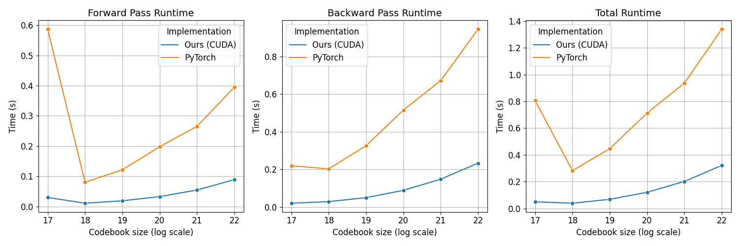
Our method is consistently 6-7x faster than the PyTorch implementation for $L = 19, 20$ (default values), showing the efficiency of the CUDA implementation for forward pass based on non-coalesced memory access.
The ablations on the desired resolution $D$ are shown below:
| Resolution | CUDA Fwd | PyTorch Fwd | CUDA Bwd | PyTorch Bwd | Fwd Speedup | Bwd Speedup |
|---|---|---|---|---|---|---|
| 32 | 0.0011 | 0.0066 | 0.0048 | 0.0076 | 5.9026 | 1.5876 |
| 48 | 0.0024 | 0.0061 | 0.0073 | 0.0104 | 2.5590 | 1.4132 |
| 64 | 0.0047 | 0.0076 | 0.0131 | 0.0194 | 1.6327 | 1.4824 |
| 96 | 0.0109 | 0.0421 | 0.0268 | 0.0971 | 3.8480 | 3.6272 |
| 128 | 0.0138 | 0.0737 | 0.0356 | 0.1778 | 5.3606 | 4.9871 |
| 196 | 0.0172 | 0.1062 | 0.0449 | 0.2726 | 6.1640 | 6.0705 |
| 256 | 0.0190 | 0.1240 | 0.0500 | 0.3269 | 6.5094 | 6.5437 |
| 384 | 0.0210 | 0.1388 | 0.0555 | 0.3859 | 6.6049 | 6.9488 |
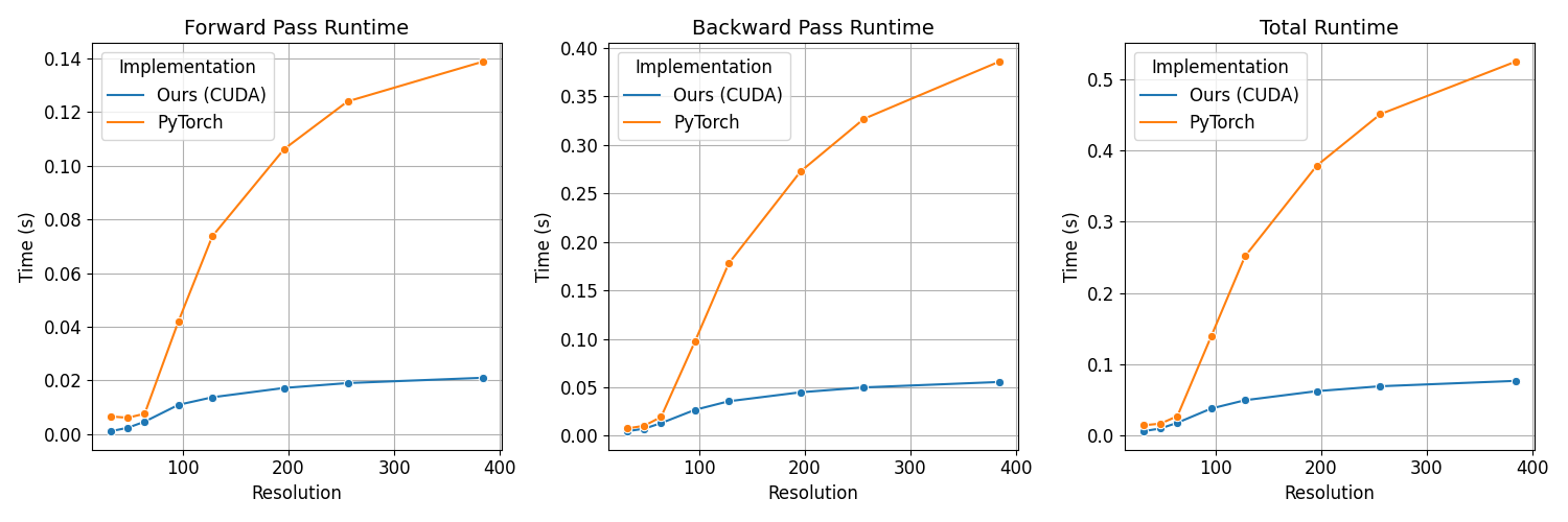
In the above table, we see that the CUDA implementation is consistently faster than the PyTorch implementation for all resolutions. The speedup is more pronounced for higher resolutions because higher desired resolutions imply more compression at the same codebook size.
Conclusion
In this blog post, we introduced NGPConv, a method for scaling 3D convolutional networks to process much larger volumes by leveraging implicit neural representations. By using Instant NGP’s hash-based encoding with shared decoders, we can represent high-resolution 3D data efficiently while maintaining spatial locality and consistent basis functions across samples. This allows us to perform convolutions directly on the compressed implicit representation rather than the full voxel grid.
Our CUDA implementation demonstrates significant speedups over a naive PyTorch implementation, achieving 6-7x faster forward passes and 4-6x faster backward passes for typical parameter settings. The performance benefits are particularly pronounced at higher resolutions, where the compression ratio is greater. This makes NGPConv practical for processing large 3D volumes that were previously intractable, like high-resolution medical imaging data or neural radiance fields.
The approach opens up new possibilities for 3D deep learning by breaking through the memory bottleneck that has traditionally limited 3D ConvNet architectures. Future work could explore applying this technique to other 3D learning tasks and further optimizing the implementation for even better performance.